
It was a very, very, boring day in late May for me. My freshman year at college had just ended two weeks ago, and it would be another two weeks before my summer classes would begin. I’m not a workaholic, but I tend to be a bit of a bum if I’m not kept busy with at least one thing. Fortunately, I wouldn’t have time to be bored because I got an email from one of my professors, asking me if I wanted to start working on a project that would create a machine learning (ML) model that would count the number of bees on a hive frame just by snapping a single picture of it (potential app idea for beekeepers once other functionalities are added). I immediately signed on and began working on putting it together.
How I Began
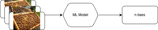
At the very beginning, I had absolutely no idea where to start. All I knew was I wanted to feed images into a machine learning model and get it to return a count of the bees, like the basic flow at the top of the article. What model I would use, how I would prepare the images to actually give to the model, and how I would figure out a workflow were all big mysteries to me at this point. But according to Lao Tzu, the journey of a thousand miles begins with a single step. And that first, single step was a Google search. I spent about 10 minutes on the web before I came across an interesting lead. On GitHub, I found a project from about 7 years ago focused on crowd counting densely populated images.
The model was a convolutional neural network, also known as a CNN, which is a specific type of neural network that has inherent hierarchies and is commonly used in image processing. It works by splitting the input image into layers that detect low-level features and then stacking them to make sense of what is created. For example, if one layer detects horizontal lines and another detects verticals, during the convolution stage, it turns those lines into an edge. Their specific model (CSRNet), instead of trying to count individual items, attempts to estimate the density of those items (which, on a side note, almost guarantees that the result will be a decimal). This project was an amazing find because while it was the first thing I found that was close to a real workflow that I could use to build my project onto, most of the beginning steps were already outlined there.

My Plan
A basic summary of my plan of action was as follows:
- Annotate the image in JPG format to mark the heads of the bees
- Make an image and annotation .h5 file pair (known as the ground truth, GT)
- Feed them into the neural network to return a .pth model that could accurately predict the number of bees.
I have to admit, the first step gave me quite a headache. I couldn’t find a good annotation software that would return the density heatmaps in the necessary format, and besides, most of them came with a hefty usage fee. Eventually, I decided to create my own small Python script whose basic functionality allowed me to open the image, click on the location of the bee, create a univariate Gaussian density distribution centered at each point, and write that density to a .h5 file.
A Gaussian distribution (named after the mathematician Carl Friedrich Gauss) is simply the normal distribution on a 2-dimensional surface. This step was important because a computer can’t use points, a zero-dimensional object, to determine a density. It needs an area in which it can do this, and the Gaussian was the first choice. An advantage of this method was that if multiple bees were overlapping, their Gaussians would be additive, meaning that the area of overlap would be counted as more dense than just a single bee. This script went through several quality-of-life updates before it was really ready to use.
    while annotating:
        key = cv2.waitKey(0)
        if key == ord('s'):
            save_image = True
            annotating = False
        elif key == ord('n'):
            skip_image = True
            annotating = False
        elif key == ord('q'):
            quit_now = True
            annotating = False
        elif key == ord('u'):
            if points:
                points.pop()
                print("Removed last point.")
                redraw_points()
            else:
                print("No points to remove.")
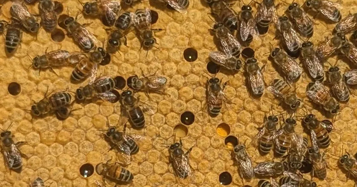
The actual annotations were not nearly as bad from a conceptual perspective, but they were incredibly tedious to do. I redid them several times because I couldn’t stop changing the images, first using the original ones, then cutting them up, and then cutting them up some more. I would like to credit my younger brothers for helping me out with this annoyingly long task. One of the things to figure out was where to mark the bee. After consulting with a friend, I decided to focus on the thorax of the bees since they were the easiest part of them to individually identify. But nevertheless, annotating was difficult because some images were incredibly dense. Sometimes we ourselves had to “predict” the number of bees in a given location, because it was absolutely impossible to count them with 100 percent confidence. Together, we ended up annotating 151 images with approximately 600×800 resolution, with bee counts ranging from the single digits to over 100.

Implementing the Model
Finally, the last step in this proof-of-concept part of the project was to actually create and run the CSRnet model. After building the baseline 3 files to create the dataset in the right format, outlining the model specs, and actually training the model, I tested it by running 11 images through 50 epochs of the CSRnet. It didn’t work, mainly because it expected images of the exact same resolution (and all mine were different because I was cutting them up with Microsoft Paint). So, I had to tweak the dataset script for the model to be able to take an image of any resolution. After running it successfully, I came back with the results, which were complete garbage. There were multiple reasons for this, but the most pressing one was the fact that I made the radius (the sigma) of the Gaussian too small, marking about 15 percent of the thorax at best. I enlarged the radius to better include the entire thorax and updated my methods of error calculation, switching from mean absolute error (MAE) to loss percentage of the bee count. After running it again with the 151 images, I definitely got … results. Not something that was anywhere near a finished model, but rather a model that performed appropriately given the number of images I fed into it. This had the potential to hit my accuracy goal (which was a minimum of 90%, with 95% being a good benchmark for my purposes).
Given that this was still in the proof-of-concept stage, I needed to figure out how exactly upscaling would look: the size of the dataset needed to train a decent model, the computing resources necessary to run the scripts in a reasonable time, any potential tweaks to the model architecture, etc… AI was incredibly useful for helping me research, and I found out that I would need several thousand images to create an acceptable dataset. Now, this put forth two problems that anyone who works on medium or large-scale machine learning models deals with almost on a daily basis. First, where to obtain that many images of beehive frames (that were all approximately 600×800)? These images would also need to be annotated, and it would take an absolutely absurd amount of time to do it by hand, given that this was an extremely limited 2-man project.
def apply_augmentations(img, dmap):
    # Horizontal flip
    if random.random() < 0.5:
        img = cv2.flip(img, 1)
        dmap = cv2.flip(dmap, 1)

    # Vertical flip
    if random.random() < 0.5:
        img = cv2.flip(img, 0)
        dmap = cv2.flip(dmap, 0)

    # Rotation
    angle = random.uniform(-MAX_ROTATE_DEG, MAX_ROTATE_DEG)
    img = rotate(img, angle, reshape=False, mode='reflect')
    dmap = rotate(dmap, angle, reshape=False, mode='reflect')

    # Brightness and contrast
    alpha = random.uniform(0.8, 1.2)
    beta = random.uniform(-10, 10)
    img = np.clip(alpha * img + beta, 0, 255).astype(np.uint8)

    return img, dmap
However, the solution to this problem was hiding just under my nose, because given the nature of the images, they would work really well with image augmentation. Augmentation is a process where one base image is slightly altered in different ways (rotation, changes to the saturation, etc.) and is multiplied to create several changed “copies”, normally to beef up a dataset. Another advantage is that I could subject the GT annotations to the same alterations, saving me from needing to reannotate them. Since I heavily augmented this dataset, I got 19 copies per image, which, when used with the originals, came out to be a dataset of 3040 images. While it is unusual at best to use an almost entirely artificial dataset, I believed it could work since the images themselves have no real concept of orientation, and the changes in the color saturation would simulate different weather conditions. But the accuracy of my predictions still needed to be tested. This brings us to the second problem: actually getting my hands on the computing resources necessary to process this dataset. I would need cloud computing resources to finish running the script within 24 hours. Without actually running the dataset, no further meaningful improvements can be made, simply due to the lack of information.
Part II coming soon….