Smash: A Visual Journey into Particle Collisions
Introduction
On a Saturday morning I was sent a link to a draft for part one of this series written by Chris King. Reading said draft resulted in possibly the most effective nerd sniping of all time.
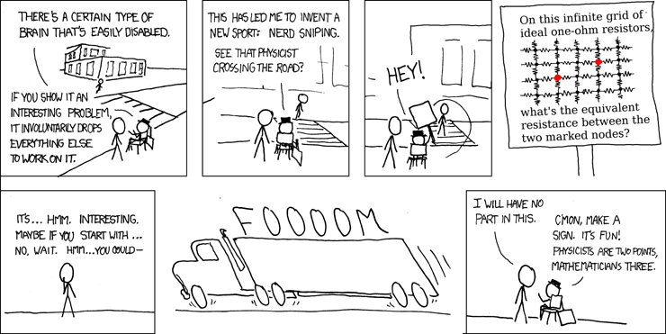
Just like that, my weekend was consumed by research. I was captivated by what happens when particles collide at high energies, and would not rest until I could simulate it for myself.
I am in no way shape or form an expert in quantum mechanics, particle physics, and/or the Standard Model. The furthest my understanding reaches is the basics of Maxwell’s equations in classical electromagnetics. With that said, let us dive into the standard model.
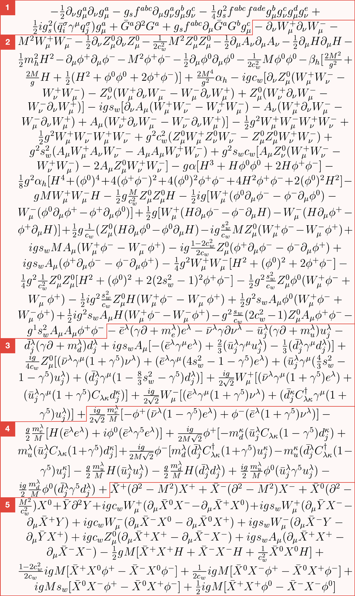
The Standard Model describes the particles which make up the universe and the fundamental forces acting upon them. The Standard Model considers 17 elementary particles in the following categories Quarks, Leptons, Gauge bosons and the Higgs boson. The quarks and leptons are considered fermions which obey the Pauli-exclusion principle and are modelled with Fermi-Dirac statistics. The bosons are force-carrier particles which do not obey the Pauli exclusion principle. The bosons model the three fundamental forces in the Standard Model: Electromagnetic Force, Weak Nuclear Force, and Strong Nuclear Force. If you want to know more about the Standard Model, there are some great resources for it here and here. For the mathletes out there, here is the Lagrangian form for describing the Standard Model:
Understanding the Standard Model is crucial for appreciating the world of particle physics and the interactions that occur at the smallest scales of matter. However, I am not satisfied with a theoretical description alone; visualizing these complex interactions is a personal requirement and one I hope a reader can appreciate. In this blog, we will explore how Pythia can be used to visualize particle collisions, offering a practical approach to studying the fundamental aspects of particle physics and enjoying the beauty within possibly natures most violent collisions. All of our code for our particle simulation work is available on GitHub at https://github.com/chrisk60331/particle_experiments/
Pythia
Pythia is a general purpose Monte Carlo event generator. It is an incredible tool for simulating high energy collisions between particles. This will be the tool used for defining the physics of the simulations we will be visualizing.
Installation
Installing Pythia requires compiling the source files. There are steps available on their website for compiling, however for the purposes of the post I am more interested in the python compatible version. There is an available wrapper for all the c++ functionality. Once you have downloaded and unzipped the tarball, open a terminal in the pythia8312 directory. To compile a Pythia version usable in python, the compilation process needs to know where the python environment is. I wanted to use a specific virtual environment, which was done with the following commands:
./configure --with-python-config=[path to python3-config file]

# if everything worked correctly you should see the following
---------------------------------------------------------------------
|                    PYTHIA Configuration Summary                   |
---------------------------------------------------------------------
  Architecture                = DARWIN
  C++ compiler     CXX        = g++
  C++ dynamic tags CXX_DTAGS  =
  C++ flags        CXX_COMMON = -O2 -std=c++11 -pedantic -W -Wall -Wshadow -fPIC -pthread
  C++ shared flag  CXX_SHARED = -dynamiclib
  Further options             =

The following optional external packages will be used:
 + PYTHON (-I/opt/homebrew/Caskroom/miniconda/base/envs/PythiaEnv/include/python3.12 -I/opt/homebrew/Caskroom/miniconda/base/envs/PythiaEnv/include/python3.12)

# now build it, this will take a little bit.
make
To test your Pythia installation, you can run one of the example scripts provided by the authors.
# main291.py is a part of the PYTHIA event generator.
# Copyright (C) 2024 Torbjorn Sjostrand.
# PYTHIA is licenced under the GNU GPL v2 or later, see COPYING for details.
# Please respect the MCnet Guidelines, see GUIDELINES for details.

# Keywords: basic usage; charged multiplicity; python;

# This is a simple test program, equivalent with main101.cc,
# but written in Python. It fits on one slide in a talk.
# It studies the charged multiplicity distribution at the LHC.

# To set the path to the Pythia 8 Python interface do either
# (in a shell prompt):
#      export PYTHONPATH=$(PREFIX_LIB):$PYTHONPATH
# or the following which sets the path from within Python.
import sys
cfg = open("Makefile.inc")
lib = "../lib"
for line in cfg:
    if line.startswith("PREFIX_LIB="): lib = line[11:-1]; break
sys.path.insert(0, lib)

#==========================================================================

# Import the Pythia module.
import pythia8
pythia = pythia8.Pythia()
pythia.readString("Beams:eCM = 8000.")
pythia.readString("HardQCD:all = on")
pythia.readString("PhaseSpace:pTHatMin = 20.")
pythia.init()
mult = pythia8.Hist("charged multiplicity", 100, -0.5, 799.5)
# Begin event loop. Generate event. Skip if error. List first one.
for iEvent in range(0, 100):
    if not pythia.next(): continue
    # Find number of all final charged particles and fill histogram.
    nCharged = 0
    for prt in pythia.event:
        if prt.isFinal() and prt.isCharged(): nCharged += 1
    mult.fill(nCharged)
# End of event loop. Statistics. Histogram. Done.
pythia.stat();
print(mult)
I prefer setting the path from within python, which just requires pointing to the Makefile.inc file in the pythia8312 folder.
Simulation
The interface to Pythia allows us to specify experiment parameters through the pythia.readString method. There is plenty of documentation available for it, but for the purposes of smashing some protons together we can use the following chunk:
energy_scale = 1
energyFactor = 2000
angle = np.pi / 24  # glancing angle
momentum_p1 = np.array([energy_scale * np.cos(angle), energy_scale * np.sin(angle), 0]) * energyFactor
momentum_p2 = np.array([-energy_scale, 0, 0]) * energyFactor

pythia = pythia8.Pythia()
pythia.readString("Beams:idA = 2212")
pythia.readString("Beams:idB = 2212")
pythia.readString("Beams:frameType = 3")
pythia.readString(f"Beams:pxA = {momentum_p1[0]}")
pythia.readString(f"Beams:pyA = {momentum_p1[1]}")
pythia.readString(f"Beams:pzA = {momentum_p1[2]}")
pythia.readString(f"Beams:pxB = {momentum_p2[0]}")
pythia.readString(f"Beams:pyB = {momentum_p2[1]}")
pythia.readString(f"Beams:pzB = {momentum_p2[2]}")

pythia.readString("HardQCD:all = on")
This will set up an experiment with two protons colliding at the defined glancing angle. Note that the energy factor variable does not directly define the energy of each particle, it scales each component of the momentum vector.
These collisions are very stochastic, so the framework is designed to simulate each event many times.
pythia.init()

for iEvent in range(nevents):
  if not pythia.next(): continue. # there was an error
  numParticles = pythia.event.size()
  # access individual particles in the event list with
  for i in range(numParticles):
    particle = pythia.event[1]
    p = particle.p(). # momentum vector
    vProd = particle.vProd()  # production vector
    tau = particle.tau(). # lifetime
    survived = particle.isFinal()  # did not decay
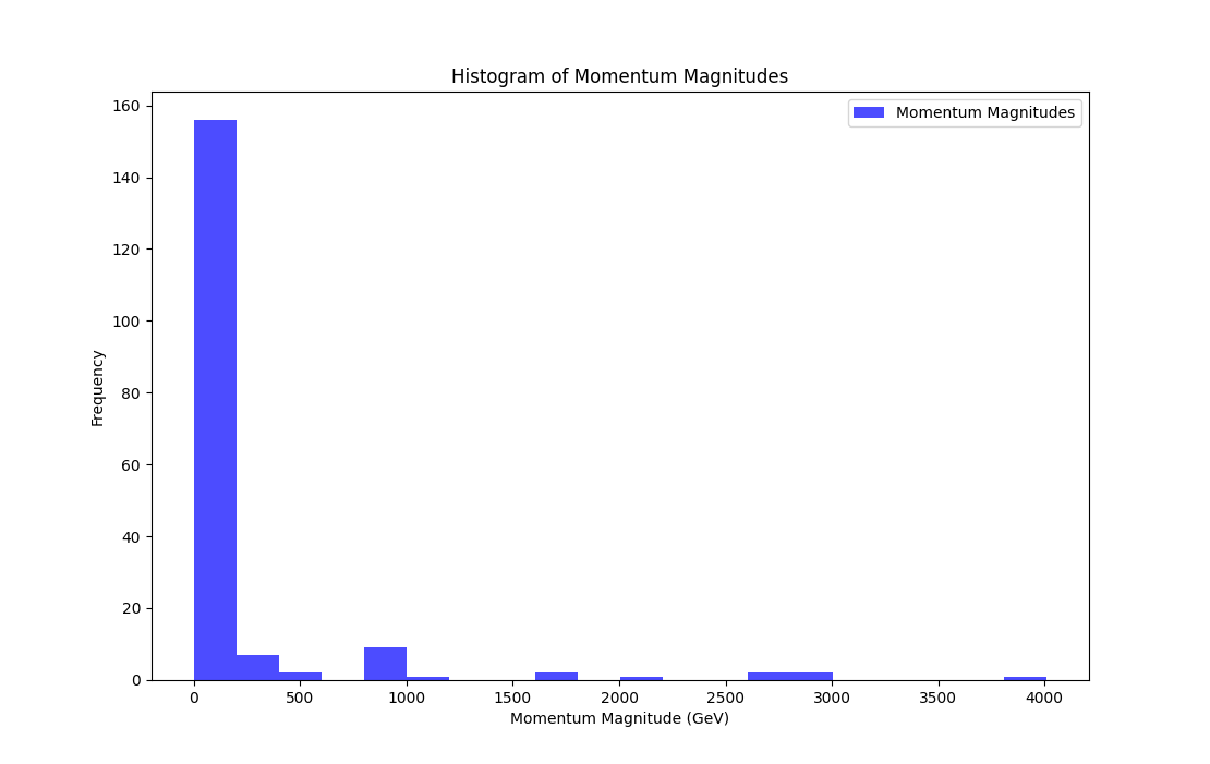
The physicists using these results are going to be mostly interested in histograms of momenta and generated particles, like these visuals:
Or even something like this:
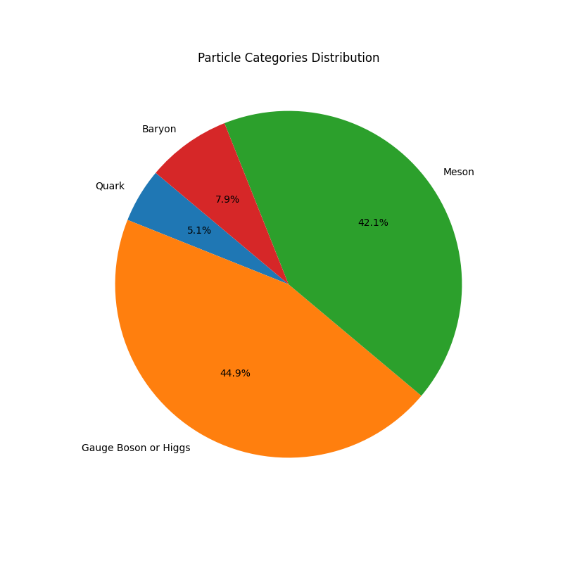
Remember I said at the start I am no physicist. Let’s build something to let us watch the collision and simply enjoy it rather than analyze it. We will need a tool that is great for visualizing point clouds, and ideally one that allows for time stepping. Vispy has an example of an n-body simulation on its front page, which immediately sold me as being the right tool for the job here.
Naive Simulation
Simulating the event will require the momentum and the starting point of each particle. A lot of the particles produced in the collision are unstable and decay almost immediately. For now, we will ignore the lifetime of particles and just visualize everything based on the starting position and shift the particles along their respective momenta.
Pythia provides all the information we require and can be accessed through their particle object.
# Begin event loop. Generate event. Skip if error. List first one.
for iEvent in range(nevents):
    if not pythia.next(): continue
    numParticles = pythia.event.size()
    if numParticles != 0:
        points_matrix = np.zeros((numParticles, 3))
        momentum_matrix = np.zeros((numParticles, 3))
        categories = np.zeros(numParticles)
        lifetimes = np.zeros(numParticles)
        spawnTimes = np.zeros(numParticles)
        id_array = np.zeros(numParticles)
        storedParticles = 0
        for i in range(numParticles):
            particle = pythia.event[i]
            print("Particle", i, "has PID = ", particle.id())
            id = particle.id()
            try:
                named_particle = NamedParticle.from_pdgid(id)
                particle_name = named_particle.name
            except Exception as e:
                # didnt find it oh well, name isnt critical
                pass

            p = particle.p(). # momentum vector
            mass = particle.m()
            vProd = particle.vProd()
            tau = particle.tau()
            survived = particle.isFinal()
            decaySpot = particle.vDec()
            # store the starting point of the particle
            points_matrix[i] = np.array([vProd[0], vProd[1], vProd[2]])
            # store the momentum of the particle
            momentum_matrix[i] = np.array([p[0], p[1], p[2]])
            id_array[i] = id
            categories[i] = categorize_particle_numerically(id)
            lifetimes[i] = tau
            spawnTimes[i] = vProd[3]
Using vProd (the production position of the particle) and the momentum, we can start to visualize the collision by stepping forward in time and shifting the position of the particles along their momentum vector.

One thing to note is some particles have massive momenta compared to others and if you visualize this linearly the momenta of the low energy particles is not noticeable. This can be dealt with by log normalizing magnitudes of the momenta.
def log_normalize_data(points_matrix, momentum_matrix, target_max=1.0):
    epsilon = 1e-9  # Small constant to ensure no log(0)

    # Calculate the magnitude of each vector
    magnitudes = np.linalg.norm(momentum_matrix, axis=1, keepdims=True)

    # Shift magnitudes to ensure all values are positive before log transformation
    shifted_magnitudes = magnitudes + epsilon

    # Apply log normalization
    log_magnitudes = np.log(shifted_magnitudes)

    # Normalize the log-transformed magnitudes to the target range [-target_max, target_max]
    max_log_magnitude = np.max(np.abs(log_magnitudes))
    normalized_magnitudes = (log_magnitudes / max_log_magnitude) * target_max

    # Recreate the momentum vectors with normalized magnitudes while preserving direction
    unit_vectors = momentum_matrix / magnitudes
    normalized_momentum_matrix = unit_vectors * normalized_magnitudes

    # normalize the points matrix linearly
    normalized_points_matrix = (points_matrix / np.max(np.abs(points_matrix))) * target_max


    return normalized_points_matrix, normalized_momentum_matrix
Each colour shown in the GIF represents a different class of particle defined in the following:
def categorize_particle_numerically(pdgid):
    pdgid_instance = PDGID(pdgid)

    # Assign a unique integer to each category
    if pdgid_instance.is_lepton:
        return 1  # Lepton
    elif pdgid_instance.is_quark:
        return 2  # Quark
    elif pdgid_instance.is_gauge_boson_or_higgs:
        return 3  # Gauge Boson or Higgs
    elif pdgid_instance.is_hadron:
        if pdgid_instance.is_meson:
            return 4  # Meson
        elif pdgid_instance.is_baryon:
            return 5  # Baryon
        else:
            return 6  # Other Hadron
    else:
        return 0  # Unknown
The colours are then produced from those categories following a jet colour map.
Decaying
As I said before, most of the particles in that simulation would have decayed almost immediately, which is not reflected above. Since most particles decay in 0 time to allow them to be visualized, I artificially changed their lifespan to give them at least 30 time steps of life. In the next simulation you will see just how many particles decay, visualized by turning purple (though the purple is tough to see against the background, so it is also like they just vanish).

I can’t speak to any of the physics behind what we just saw, but it most definitely fulfilled my need for visualizing the result of a proton-proton collision.
Conclusion
While the visualizations above may not be of any scientific value, they are fascinating to watch unfold. They offer a glimpse into the chaotic beauty of particle collisions, transforming abstract concepts into something tangible and mesmerizing. These simulations underscore the incredible complexity and elegance inherent in the Standard Model, even for those of us who are not physicists.
Through tools like Pythia and Vispy, we can appreciate the delicate interplay of forces and particles at a level that goes beyond equations and theories. By visualizing these interactions, we not only enhance our understanding but also spark curiosity and wonder about the fundamental workings of our universe.
Thank you for joining me on this adventure. Happy colliding!


