Exploring Particle Physics Simulations in Python

Editors note:

At New Math Data we strive to regularly push the envelope, test our skills, and generally innovate, in addition to a deep commitment to our more traditional practices such as analytics and data warehousing. It is in that spirit that we present this article, an experiment in data modeling, where we ask the question “can we model both the Standard Model of particle physics and elements of String Theory in an idiomatic language?”

Introduction

Particle physics, the cornerstone of our understanding of the universe’s fundamental structure, is a field that unravels the intricate behaviors and interactions of the smallest known particles. From quarks and gluons to electrons and neutrinos, the myriad particles governed by the Standard Model exhibit complex dynamics that are pivotal to the fabric of our reality. Simulating these interactions not only allows us to predict particle behavior but also to visualize phenomena that are otherwise beyond the reach of direct observation.

In this blog post, we embark on a journey to construct a particle physics simulation using Python. Our goal is to model the forces at play, simulate particle interactions such as decay, collisions, and scattering, and visualize their trajectories. By leveraging the power of computational simulations, we can gain insights into particle dynamics that enhance our theoretical and practical understanding of the subatomic world.

For on-going updates, follow our GitHub repo.

We will begin by laying the groundwork with the implementation of particle and field classes, followed by detailing the methods to simulate interactions. Next, we will delve into the dynamics of running the simulation and updating particle states. Finally, we will visualize the trajectories of these particles to better understand their interactions and behaviors. Join us as we explore the fascinating world of particle physics through the lens of computational simulations.

Building the Foundation – Particle and Field Classes

Defining Particles

At the heart of our simulation lies the Particle class, a blueprint for the various particles we aim to model. Each particle is characterized by fundamental properties such as mass, charge, spin, and velocity. These attributes are not just numerical values; they determine how particles interact with each other and with fields.

The Particle class encapsulates these properties and provides methods to compute derived quantities like energy and momentum. The mass of a particle, measured in MeV/c², dictates its resistance to acceleration. Charge, expressed in elementary charge units (e), determines how the particle responds to electric and magnetic fields. Spin, a quantum mechanical property, influences the particle’s statistical behavior and interaction dynamics.

class Particle:
    def __init__(
        self,
        name,
        symbol,
        mass,
        charge,
        spin,
        string_mode,
        decay_constant=0.0,
        decays_to=None,
        velocity=None,
    ):
        self.name = name
        self.symbol = symbol
        self.mass = mass
        self.charge = charge
        self.spin = spin
        self.string_mode = string_mode
        self.decay_constant = decay_constant
        self.decays_to = decays_to if decays_to else []
        self.velocity = (
            velocity
            if velocity
            else (
                random.uniform(-0.5 * c, 0.5 * c),
                random.uniform(-0.5 * c, 0.5 * c),
            )
        )
        self.energy = self.calculate_energy()
        self.momentum = self.calculate_momentum()
        self.positions = [(0, 0)]  # Store positions for visualization

    def __repr__(self):
        return f"{self.name} ({self.symbol}): Mass={self.mass} MeV/c^2, Charge={self.charge}e, Spin={self.spin}, String Mode={self.string_mode}, Velocity={self.velocity}, Energy={self.energy} MeV, Momentum={self.momentum} MeV/c"

Velocity is a vector quantity representing the particle’s motion through space. To handle relativistic effects, the class includes methods to calculate the Lorentz factor, ensuring that velocities approach but do not exceed the speed of light (c). By integrating these properties, the Particle class forms the cornerstone of our simulation, enabling realistic modeling of particle behavior.

def lorentz_factor(self):
    vx, vy = self.velocity
    speed_squared = vx**2 + vy**2
    if self.mass == 0:
        return 1
    if speed_squared >= c**2:
        speed_squared = c**2 * 0.99
    return 1 / math.sqrt(1 - speed_squared / c**2)

def calculate_energy(self):
    vx, vy = self.velocity
    speed_squared = vx**2 + vy**2
    if self.mass == 0:
        return math.sqrt(speed_squared) * c
    gamma = self.lorentz_factor()
    return gamma * self.mass * c**2

def calculate_momentum(self):
    vx, vy = self.velocity
    speed_squared = vx**2 + vy**2
    if self.mass == 0:
        energy = math.sqrt(speed_squared) * c
        return (
            vx / math.sqrt(speed_squared) * energy / c,
            vy / math.sqrt(speed_squared) * energy / c,
        )
    gamma = self.lorentz_factor()
    return gamma * self.mass * vx, gamma * self.mass * vy

Modeling Fields

To simulate particle interactions accurately, we must consider the forces exerted by electric and magnetic fields. The ElectricField and MagneticField classes model these influences using the Lorentz force law.

The ElectricField class applies a constant electric field to particles, resulting in a force proportional to the particle’s charge and the field strength. This force induces acceleration, altering the particle’s velocity over time. The apply method updates the particle’s velocity vector, taking into account the time step of the simulation.

class ElectricField:
    def __init__(self, field_strength):
        self.field_strength = field_strength

    def apply(self, particle, time_step):
        force_x = particle.charge * self.field_strength[0]
        force_y = particle.charge * self.field_strength[1]

        if particle.mass > 0:
            ax = force_x / particle.mass
            ay = force_y / particle.mass

            new_vx = particle.velocity[0] + ax * time_step
            new_vy = particle.velocity[1] + ay * time_step
            particle.update_velocity(new_vx, new_vy)

Similarly, the MagneticField class models the effects of a magnetic field. The Lorentz force in this context is given by the cross product of the particle’s velocity and the magnetic field vector, scaled by the particle’s charge. This results in a perpendicular force that changes the particle’s trajectory without altering its speed. The apply method calculates this force and updates the particle’s velocity accordingly.

class MagneticField:
    def __init__(self, field_strength):
        self.field_strength = field_strength

    def apply(self, particle, time_step):
        vx, vy = particle.velocity
        Bz = self.field_strength[2]
        force_x = particle.charge * vy * Bz
        force_y = -particle.charge * vx * Bz

        if particle.mass > 0:
            ax = force_x / particle.mass
            ay = force_y / particle.mass

            new_vx = particle.velocity[0] + ax * time_step
            new_vy = particle.velocity[1] + ay * time_step
            particle.update_velocity(new_vx, new_vy)

Together, these classes provide a framework for simulating the dynamic interactions between particles and fields. By updating particle velocities and positions in response to these forces, we can capture the intricate dance of particles under the influence of electromagnetic fields, laying the foundation for more complex simulations.

Implementing Interactions – Decay, Collision, and Scattering

Particle Decay

Particle decay is a fundamental process in particle physics where unstable particles transform into other particles over time. This transformation is probabilistic in nature, governed by decay constants unique to each particle. In our simulation, the decay method models this behavior.

The method first checks if the particle has a non-zero decay constant. It then calculates the probability of decay occurring within the given time step using an exponential decay law. If decay occurs, the particle is replaced by its decay products, distributing the energy and momentum among them. This is crucial for accurately modeling particle lifetimes and the resultant particles from decays.

def decay(self, time_step):
    if self.decay_constant == 0:
        return [self]
    decay_probability = 1 - math.exp(-self.decay_constant * time_step)
    if random.random() < decay_probability:
        decay_products = random.choice(self.decays_to)
        total_energy = self.energy
        total_momentum = self.momentum
        num_products = len(decay_products)
        for product in decay_products:
            product.energy = total_energy / num_products
            product.momentum = (
                total_momentum[0] / num_products,
                total_momentum[1] / num_products,
            )
            if product.mass != 0:
                p_velocity_magnitude = math.sqrt(
                    (product.momentum[0] ** 2 + product.momentum[1] ** 2)
                    / product.mass**2
                )
                if p_velocity_magnitude >= c:
                    scale = (c * 0.99) / p_velocity_magnitude
                    p_velocity_magnitude *= scale
                product.update_velocity(
                    product.momentum[0] / product.mass,
                    product.momentum[1] / product.mass,
                )
            else:
                product.velocity = (
                    product.momentum[0] / product.energy * c,
                    product.momentum[1] / product.energy * c,
                )
        print(
            f"{self.name} decays into {', '.join([p.symbol for p in decay_products])}"
        )
        return decay_products
    else:
        return [self]

Collisions and Annihilation

Collisions between particles are another critical aspect of particle interactions. When two particles collide, they can form a new particle with combined mass and charge. The collide method handles this by creating a new particle and determining its properties based on the colliding particles.

Annihilation occurs when a particle meets its antiparticle, resulting in their mutual destruction and the creation of photons. This process is modeled in the annihilate method, which checks for charge neutrality and generates photon products accordingly.

def collide(self, other):
    new_mass = self.mass + other.mass
    new_charge = self.charge + other.charge
    new_velocity = (
        (self.velocity[0] + other.velocity[0]) / 2,
        (self.velocity[1] + other.velocity[1]) / 2,
    )
    new_particle = Particle(
        f"NewParticle({self.symbol}+{other.symbol})",
        f"{self.symbol}{other.symbol}",
        new_mass,
        new_charge,
        0,
        "mode_new",
        velocity=new_velocity,
    )
    print(
        f"{self.name} and {other.name} collide to form {new_particle.name}"
    )
    return new_particle

def annihilate(self, other):
    if self.charge + other.charge == 0:
        total_energy = self.energy + other.energy
        photon1 = Particle(
            "Photon", "γ", 0, 0, 1, "mode_γ", velocity=(c, 0)
        )
        photon2 = Particle(
            "Photon", "γ", 0, 0, 1, "mode_γ", velocity=(-c, 0)
        )
        photon1.energy = total_energy / 2
        photon2.energy = total_energy / 2
        print(
            f"{self.name} and {other.name} annihilate to form two photons"
        )
        return [photon1, photon2]
    else:
        return [self, other]

Scattering Events

Scattering events occur when particles interact and exchange velocities without forming new particles. This is common in high-energy physics where particles deflect off each other due to their electric charges. The scatter method models this by swapping the velocities of the interacting particles, thus simulating the scattering process.

def scatter(self, other):
    self_velocity = self.velocity
    other_velocity = other.velocity
    self.update_velocity(*other_velocity)
    other.update_velocity(*self_velocity)
    print(f"{self.name} and {other.name} scatter, exchanging velocities")

Integration of Interactions in the Simulation

To incorporate these interactions into our simulation, the simulate_interactions function checks for possible decays, collisions, and scattering at each time step. It updates the state of each particle accordingly, ensuring a realistic representation of particle dynamics.

def simulate_interactions(particles, fields, steps):
    for step in range(steps):
        print(f"\nStep {step + 1}")

        particles_copy = particles[:]
        interactions_done = set()
        for i in range(len(particles_copy)):
            for j in range(i + 1, len(particles_copy)):
                p1 = particles_copy[i]
                p2 = particles_copy[j]
                if (p1, p2) in interactions_done or (
                    p2,
                    p1,
                ) in interactions_done:
                    continue
                interactions_done.add((p1, p2))
                if p1.charge + p2.charge == 0 and random.random() < 0.1:
                    new_particles = p1.annihilate(p2)
                    particles.extend(new_particles)
                    if p1 in particles:
                        particles.remove(p1)
                    if p2 in particles:
                        particles.remove(p2)
                elif random.random() < 0.1:
                    new_particle = p1.collide(p2)
                    particles.append(new_particle)
                    if p1 in particles:
                        particles.remove(p1)
                    if p2 in particles:
                        particles.remove(p2)
                elif random.random() < 0.1:
                    p1.scatter(p2)

        for field in fields:
            for particle in particles:
                field.apply(particle, 1 / steps)

        for particle in particles[:]:
            new_vx = particle.velocity[0] + random.uniform(-0.01 * c, 0.01 * c)
            new_vy = particle.velocity[1] + random.uniform(-0.01 * c, 0.01 * c)
            particle.update_velocity(new_vx, new_vy)
            particle.update_position(1 / steps)
            decay_products = particle.decay(1 / steps)
            if decay_products != [particle]:
                particles.remove(particle)
                particles.extend(decay_products)

        print("Current particles:")
        for particle in particles:
            print(particle)

By accurately modeling decays, collisions, and scattering events, our simulation captures the complex interactions that define particle physics. This sets the stage for visualizing these dynamics and gaining deeper insights into the behavior of fundamental particles.

Simulating Particle Dynamics

Setting Up the Simulation

To effectively simulate particle interactions, we must initialize the simulation with a diverse set of particles and the fields that influence them. Our initial setup includes defining particles like electrons, protons, muons, and various neutrinos, each with specific properties such as mass, charge, and initial velocity. Additionally, we establish the electric and magnetic fields that will act upon these particles.

def simulate():
    electron = Particle(
        "Electron",
        "e",
        0.511,
        -1,
        1 / 2,
        "mode_1",
        velocity=(0.1 * c, 0.2 * c),
    )
    electron_neutrino = Particle(
        "Electron Neutrino",
        "νe",
        0.0000022,
        0,
        1 / 2,
        "mode_2",
        velocity=(0.1 * c, 0.2 * c),
    )
    muon_neutrino = Particle(
        "Muon Neutrino",
        "νμ",
        0.17,
        0,
        1 / 2,
        "mode_3",
        velocity=(0.1 * c, 0.2 * c),
    )
    tau_neutrino = Particle(
        "Tau Neutrino",
        "ντ",
        15.5,
        0,
        1 / 2,
        "mode_4",
        velocity=(0.1 * c, 0.2 * c),
    )
    muon = Particle(
        "Muon",
        "μ",
        105.66,
        -1,
        1 / 2,
        "mode_5",
        0.1,
        decays_to=[[electron, electron_neutrino, muon_neutrino]],
        velocity=(0.05 * c, 0.1 * c),
    )
    tau = Particle(
        "Tau",
        "τ",
        1776.86,
        -1,
        1 / 2,
        "mode_6",
        0.2,
        decays_to=[[muon, muon_neutrino, tau_neutrino]],
        velocity=(0.01 * c, 0.02 * c),
    )
    photon = Particle("Photon", "γ", 0, 0, 1, "mode_7", velocity=(c, c))
    proton = Particle(
        "Proton", "p", 938.27, 1, 1 / 2, "mode_8", velocity=(0.1 * c, 0.2 * c)
    )
    graviton = Particle(
        "Graviton", "G", 0, 0, 2, "mode_9", velocity=(0.5 * c, 0.5 * c)
    )
    axion = Particle(
        "Axion", "a", 1e-5, 0, 0, "mode_10", velocity=(0.05 * c, 0.1 * c)
    )
    particles = [electron, proton, tau, muon, photon, graviton, axion]
    fields = [ElectricField((1e5, 0)), MagneticField((0, 0, 1))]
    steps = 10

    print("Simulating interactions between particles in fields:")
    simulate_interactions(particles, fields, steps)
    visualize_particles(particles)

if __name__ == "__main__":  # pragma: no cover
    simulate()

Running the Simulation

The core of our simulation lies in the simulate_interactions function, which orchestrates the interactions between particles and their response to fields over multiple time steps. This function iterates through a predefined number of steps, updating particle states at each step.

During each iteration, the simulation checks for possible interactions between particles, such as decay, collision, and scattering. Fields are applied to each particle, updating their velocities according to the forces exerted. The particles' positions are also updated to reflect their movement through space.

def simulate_interactions(particles, fields, steps):
    for step in range(steps):
        print(f"\nStep {step + 1}")

        particles_copy = particles[:]
        interactions_done = set()
        for i in range(len(particles_copy)):
            for j in range(i + 1, len(particles_copy)):
                p1 = particles_copy[i]
                p2 = particles_copy[j]
                if (p1, p2) in interactions_done or (
                    p2,
                    p1,
                ) in interactions_done:
                    continue
                interactions_done.add((p1, p2))
                if p1.charge + p2.charge == 0 and random.random() < 0.1:
                    new_particles = p1.annihilate(p2)
                    particles.extend(new_particles)
                    if p1 in particles:
                        particles.remove(p1)
                    if p2 in particles:
                        particles.remove(p2)
                elif random.random() < 0.1:
                    new_particle = p1.collide(p2)
                    particles.append(new_particle)
                    if p1 in particles:
                        particles.remove(p1)
                    if p2 in particles:
                        particles.remove(p2)
                elif random.random() < 0.1:
                    p1.scatter(p2)

        for field in fields:
            for particle in particles:
                field.apply(particle, 1 / steps)

        for particle in particles[:]:
            new_vx = particle.velocity[0] + random.uniform(-0.01 * c, 0.01 * c)
            new_vy = particle.velocity[1] + random.uniform(-0.01 * c, 0.01 * c)
            particle.update_velocity(new_vx, new_vy)
            particle.update_position(1 / steps)
            decay_products = particle.decay(1 / steps)
            if decay_products != [particle]:
                particles.remove(particle)
                particles.extend(decay_products)

        print("Current particles:")
        for particle in particles:
            print(particle)

Monitoring Particle Evolution

Accurately capturing the evolution of each particle is critical to our simulation's fidelity. As particles move and interact, their velocities and positions are updated. These updates reflect changes due to forces from electric and magnetic fields, as well as interactions with other particles.

The update_velocity and update_position methods of the Particle class handle these updates. The update_velocity method ensures that particle speeds remain within relativistic limits, while the update_positionmethod tracks particle positions over time, enabling us to visualize their trajectories later.

def update_velocity(self, vx, vy):
    speed_squared = vx**2 + vy**2
    if speed_squared >= c**2:
        scale = math.sqrt(c**2 * 0.99 / speed_squared)
        vx *= scale
        vy *= scale
    self.velocity = (vx, vy)
    self.energy = self.calculate_energy()
    self.momentum = self.calculate_momentum()

def update_position(self, time_step):
    x, y = self.positions[-1]
    vx, vy = self.velocity
    new_x = x + vx * time_step
    new_y = y + vy * time_step
    self.positions.append((new_x, new_y))

By meticulously updating the state of each particle and accurately simulating their interactions, we lay the groundwork for visualizing particle dynamics. This approach allows us to observe the complex behaviors and interactions of particles as they move through space and interact with fields and each other.

Visualizing Particle Trajectories

Importance of Visualization in Particle Physics

Visualizing particle interactions is crucial for understanding the complex behaviors and dynamics that occur at the subatomic level. By observing the trajectories of particles, we can gain insights into how they move, interact, and change over time. Visualization transforms abstract data into a tangible form, making it easier to interpret and analyze the results of our simulations.

In particle physics, visualization helps bridge the gap between theoretical models and experimental observations. It allows researchers to validate their simulations against real-world data and provides a powerful tool for communicating findings within the scientific community and to the broader public.

Implementing Visualization

To visualize particle trajectories, we use the matplotlib library, a versatile tool for creating static, animated, and interactive plots in Python. Our approach involves plotting the positions of particles over time, resulting in a graphical representation of their paths through space.

We begin by defining a visualize_particles function, which takes a list of particles as input and generates a 2D plot of their trajectories. This function iterates through each particle's stored positions and plots them on a graph.

import matplotlib.pyplot as plt

def visualize_particles(particles):
    fig, ax = plt.subplots()
    for particle in particles:
        positions = zip(*particle.positions)
        ax.plot(*positions, label=particle.symbol)
    ax.set_xlabel("X Position (m)")
    ax.set_ylabel("Y Position (m)")
    ax.set_title("Particle Trajectories")
    ax.legend()
    plt.show()

In the visualize_particles function, we create a new figure and axis using plt.subplots(). We then iterate over the particles, extracting their positions and plotting them using ax.plot(). Each particle is labeled with its symbol for easy identification. Finally, we set the axis labels and title, and display the legend and plot.

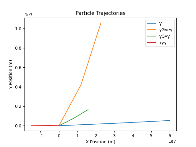
Example Visualization

Let's walk through an example to illustrate how our visualization works. Consider a simulation with particles such as electrons, protons, and photons moving under the influence of electric and magnetic fields. After running the simulation, we call the visualize_particles function to generate a plot of their trajectories.

def simulate():
    electron = Particle(
        "Electron",
        "e",
        0.511,
        -1,
        1 / 2,
        "mode_1",
        velocity=(0.1 * c, 0.2 * c),
    )
    proton = Particle(
        "Proton", "p", 938.27, 1, 1 / 2, "mode_8", velocity=(0.1 * c, 0.2 * c)
    )
    photon = Particle("Photon", "γ", 0, 0, 1, "mode_7", velocity=(c, c))
    particles = [electron, proton, photon]
    fields = [ElectricField((1e5, 0)), MagneticField((0, 0, 1))]
    steps = 10

    print("Simulating interactions between particles in fields:")
    simulate_interactions(particles, fields, steps)
    visualize_particles(particles)

if __name__ == "__main__":  # pragma: no cover
    simulate()

Running this simulation, we can observe the paths of the electron, proton, and photon as they move through the fields and interact with each other. The resulting plot provides a clear visual representation of their trajectories, helping us understand how the electric and magnetic forces influence their motion.

By implementing and utilizing visualization techniques, we transform our simulation data into a format that is easy to analyze and interpret. This enables us to gain deeper insights into particle dynamics and enhances our ability to communicate our findings effectively.

Conclusion

Simulating and visualizing particle interactions offers invaluable insights into the fundamental processes that govern the universe. By leveraging Python to model particles and their interactions with electric and magnetic fields, we can observe the complex behaviors of particles, including decays, collisions, and scattering events. Visualization using matplotlibtransforms our simulations into tangible representations, making it easier to interpret and analyze the results. This approach not only enhances our understanding of particle physics but also demonstrates the power of computational tools in advancing scientific research. As we continue to refine our simulations, we move closer to uncovering the mysteries of the subatomic world.