Introduction

In this blog post we will introduce vector databases and some of the algorithms used for indexing and show examples of how to work with AWS OpenSearch vector database using python and LangChain library.

Vector databases

A vector database is a type of database that stores high-dimensional vectors for fast retrieval and similarity search. These vectors are mathematical representations of data. Each vector has a certain number of dimensions, (up to thousands), depending on the complexity and granularity of the data. The vectors are usually generated by applying transformation or embedding functions to the raw data, such as text, images, video etc.

How working process is organized with vector databases

When working with vector databases, the process is organized in following way:

• Once the input data is transformed into embedding vectors — the next step is Indexing. To increase the performance of the search, a special data structure is built on top of dataset embeddings. This data structure is called an index. Indexes are part of a vector database and Indexing means storing data in a specific way (for example using graph or clustering algorithms discussed below).
• After all vectors are indexed and stored in vector database, we can start Searching or running search queries against it.The vector database compares the indexed query vector to the indexed vectors in the dataset to find the k nearest neighbours (applying a similarity metric used by that index).
• In some cases, the vector database post-processes the search results to return the final results. Post-processing step can include filtering or re-ranking the nearest neighbours using a different similarity metric.

Challenge when searching

Let’s look at the search operation closely: given a set of vectors and a query vector, find the k nearest vectors in the set to the query. The brute force solution: for each vector in the set, compute its distance from the query vector and keep track of the top k along the way. This is the k-NN algorithm.

How the distance between vectors is calculated.

When there are millions of high-dimensional vectors in the database it can significantly increase runtime search latency. To overcome this problem Approximate k-NN search was introduced.

Approximate k-NN search

• Reduce the search scope.
• Reduce the vectors’ dimensionality.

Trade-offs of Approximate k-NN search

• Indexing takes longer
• More space is used at query time
• Accuracy of results is worse (100% accurate results are not guaranteed)

Some of the indexing algorithms for Approximate k-NN search

There are lots of existing indexing algorithm for Approximate k-NN search. I am covering two of them (supported by AWS OpenSearch) in this blog. Those two are HNSW and IVF.

HNSW ANN algorithm

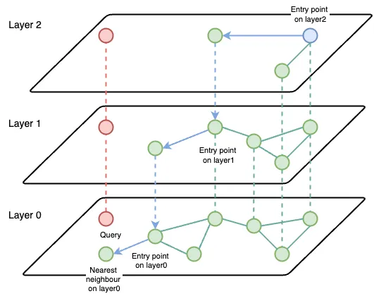
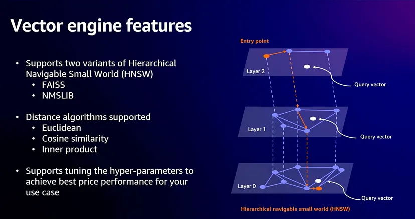
The Hierarchical Navigable Small World (HNSW) algorithm solves the latency problem by reducing the search scope. The main idea is to construct a graph where a path between any pair of vertices could be traversed in a small number of steps.

The vertex is an embedding vector. Every embedding vector has connections to the m most similar vectors.

The final structure represents a multi-layered graph with fewer connections on the top layers, more dense regions on the bottom layers and all the vectors on the lowest level.

The search starts from the highest layer and proceeds to one level below every time the local nearest neighbour is found at the current layer. Finally, the found nearest neighbour on the lowest layer is the answer to the query.

IVF ANN algorithm

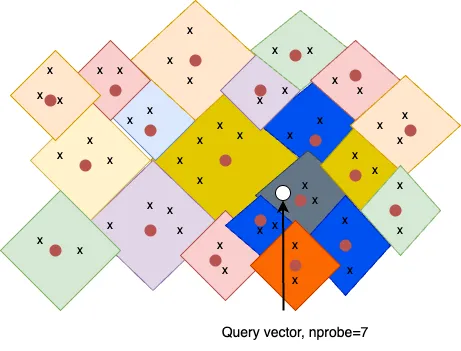
The Inverted File Index (IVF) indexing algorithm reduces search scope through clustering. Clustering can be implemented differently, one of the examples are Voronoi diagrams, also called Dirichlet tessellation.

Let’s imagine highly-dimensional embedding vectors placed into a 2D space. Every vector will be contained within a Voronoi diagrams (cell ) and every cell will have a centroid.

For the search query vector we check which cell it lands on and restrict our search scope only to that single cell. There can be a problem if search query vector falls near the edge of a cell: there is a chance that its closest other vector is contained within a neighbouring cell. This is called the edge problem.

To mitigate this problem there is a parameter called nprobe . With nprobe we can set the number of neighbour cells to search. Increasing nprobe increases the search scope.

AWS OpenSearch

According to AWS documentation:

OpenSearch by default supports Approximate k-NN Search powered by NMSLIB, FAISS and LUCENE engines recommended for large datasets. Also supports brute force k-NN search through Script Scoring and Painless Scripting.

Non-Metric Space Library (NMSLIB) — NMSLIB implements the HNSW ANN algorithm

Facebook AI Similarity Search (FAISS) — FAISS implements both HNSW and IVF ANN algorithms

Lucene — Lucene implements the HNSW algorithm

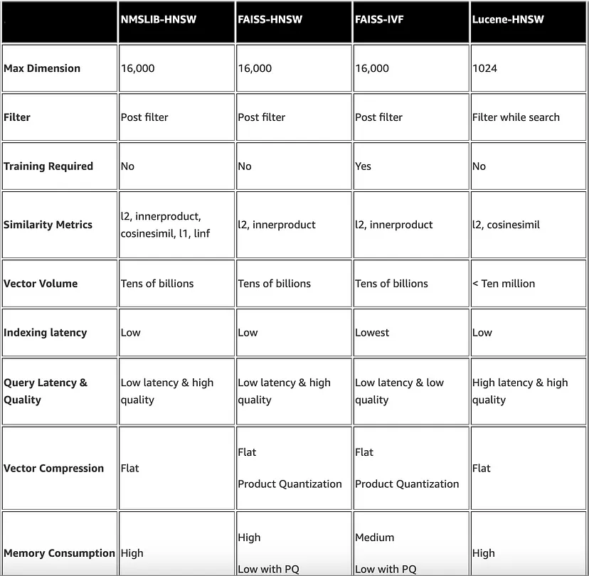
In general, NMSLIB and FAISS should be selected for large-scale use cases. Lucene is a good option for smaller deployments, but offers benefits like smart filtering where the optimal filtering strategy — pre-filtering, post-filtering, or exact k-NN — is automatically applied depending on the situation. The following table summarizes the differences between each option.

AWS OpenSearch Serverless

According to AWS Documentation:

Amazon OpenSearch Serverless is an on-demand serverless configuration for Amazon OpenSearch Service. Serverless removes the operational complexities of provisioning, configuring, and tuning the OpenSearch clusters.

For now(Apr 2024) OpenSearch Serverless supports only FAISS and NMSLIB based on HNSW and does not support IVF and IVFQ.(Documentation link).

Working with AWS OpenSearch using python LangChain library

LangChain is a popular framework for developing applications powered by large language models. Below are some code examples for how it can be used to work with AWS OpenSearch.

Note: all the examples are based on Approximate k-NN search. Brute force k-NN search is also available using Painless extensions and Script Scoring , documentation link (not covered in this blogpost).Filtering is also not covered.

Import library:

from langchain_community.vectorstores import OpenSearchVectorSearch

Preparations steps for input data:

from langchain.text_splitter import CharacterTextSplitter
from langchain_community.embeddings import BedrockEmbeddings
from langchain_community.document_loaders import UnstructuredFileLoader

files = [
    os.path.join(files_prefix, file_path)
    for file_path in os.listdir(files_prefix)
]
loader = UnstructuredFileLoader(files)
documents = loader.load()
text_splitter = CharacterTextSplitter(chunk_size=1000, chunk_overlap=0)
docs = text_splitter.split_documents(documents)
embeddings = BedrockEmbeddings(region_name=REGION_NAME)

Create new index from documents and embeddings:

docsearch = OpenSearchVectorSearch.from_documents(
    docs,
    embeddings,
    # begin - vectorsearch specific parameters
    engine="faiss",
    space_type="innerproduct",
    ef_construction=256,
    m=48,
    # end- vectorsearch specific parameters
    opensearch_url=OS_URL,
    index_name=INDEX_NAME,
    http_auth=awsauth,
    connection_class=RequestsHttpConnection,
    timeout=300,
    use_ssl=True,
    verify_certs=True,
    ssl_assert_hostname=False,
    ssl_show_warn=False,
)

Keyword Args for Approximate Search:

(From LangChain documentation)

• engine: “nmslib”, “faiss”, “lucene”; default: “nmslib”
• space_type: “l2”, “l1”, “cosinesimil”, “linf”, “innerproduct”; default: “l2”
• ef_search: Size of the dynamic list used during k-NN searches. Higher values lead to more accurate but slower searches; default: 512
• ef_construction: Size of the dynamic list used during k-NN graph creation. Higher values lead to more accurate graph but slower indexing speed; default: 512
• m: Number of bidirectional links created for each new element in the graph. Large impact on memory consumption. Between 2 and 100; default: 16
• is_appx_search: True by default, set to False to perform brute-force k-NN search

To get existing index:

docsearch = OpenSearchVectorSearch(
 embedding_function=embeddings,
 opensearch_url=OS_URL,
 index_name=INDEX_NAME,
 http_auth=awsauth,
 connection_class=RequestsHttpConnection,
 timeout=300,
 use_ssl=True,
 verify_certs=True,
 )

To perform Approximate k-NN search on the index:

query="Test question"
docsearch.similarity_search(query, k=10)

To perform Approximae k-NN search with MMR

Maximal Marginal Relevance is an additional feature supported by OpenSearch, it insures a balance between relevancy and diversity in the items retrieved. We retrieving most relevant items but these items will not be similar to each other (when using MMR)

query = "Test question"
docs = docsearch.max_marginal_relevance_search(query, k=2, fetch_k=10, lambda_param=0.5)

Keyword Args

(From LangChain documentation)

• query: text to look up documents similar to.
• k : number of Documents to return. Defaults to 4.
• fetch_k : number of Documents to fetch to pass to MMR algorithm.
• lambda_mult : number between 0 and 1 that determines the degree of diversity among the results with 0 corresponding to maximum diversity and 1 to minimum diversity. Defaults to 0.5.

Preparing model:

from langchain.chains import RetrievalQA

llm_claude = Bedrock(
        model_id="anthropic.claude-v2",
        client=bedrock_client,
        model_kwargs={"max_tokens_to_sample": 5000, "temperature": 0.1},
    )
prompt_template = "<prompt>"

Using OpenSearch vectorsearch as a retriever in RAG example1(ANN):

qa = RetrievalQA.from_chain_type(
 llm=llm_claude,
 chain_type=”stuff”,
 retriever=docsearch.as_retriever(
 search_kwargs={"k": 5}),
 return_source_documents=True,
 chain_type_kwargs={"prompt": prompt},
 )
query = "Test query"
result = qa({"query": query})

Using OpenSearch Vectorsearch as a retriever in RAG example2(MMR):

qa = RetrievalQA.from_chain_type(
 llm=llm_claude,
 chain_type=”stuff”,
 retriever=docsearch.as_retriever(
 search_type=”mmr”,
 search_kwargs={‘k’: 5, ‘fetch_k’: 30}
 ),
 return_source_documents=True,
 chain_type_kwargs={"prompt": prompt},
 )
query = "Test query"
result = qa({"query": query})

Keyword Args:

(From LangChain Documentation)

• search_type: defines the type of search that the Retriever should perform. Can be “similarity” (default), “mmr”, or “similarity_score_threshold”.
• search_kwargs: keyword arguments to pass to the search function. Can include things like:
  – k: Amount of documents to return (Default: 4)
  – score_threshold: Minimum relevance threshold for similarity_score_threshold
  – fetch_k: Amount of documents to pass to MMR algorithm (Default: 20)
  – lambda_mult: Diversity of results returned by MMR; 1 for minimum diversity and 0 for maximum. (Default: 0.5)
  – filter: Filter by document metadata

Conclusion

In this blog post I gave an introduction to vector databases and some of the indexing algorithms. I also showed some examples of how to work with AWS OpenSearch using python LangChain library. Hope you learned something. Please post your questions or comments below!