


Automating Teradata to Amazon Redshift Migration: A Practical Implementation Guide

This is a how-to article about migrating from Teradata to Redshift with a lot of technical detail based on my experience doing just that. We hope this is useful for your work, and we encourage you to post any questions in the comments section.
This article will address three key topics:
- Building a custom migration framework beyond standard AWS tools
- Advanced techniques for handling complex data types and constraints
- Implementing secure, scalable data movement with AWS Glue and Spark
While AWS offers tools like Database Migration Service (DMS) and Schema Conversion Tool (SCT) for database migrations, complex enterprise scenarios often require more control and customization. Migrating from Teradata to Amazon Redshift presents unique challenges, particularly when handling complex data types, constraints, and large-scale data movement. This article details implementation of a custom migration script that bypasses conventional tools in favor of a more flexible, powerful approach.
This approach could make sense, if you need to maintain precise control over data type mappings and transformations. Source data requires complex pre-processing before migration. You have specific requirements that DMS cannot meet or require custom error handling and validation logic.
Implementation Steps
The implementation uses PySpark for data processing and handles schema conversion, data type mapping, and constraint preservation.
1. Interactive Session & Dynamic Configuration
The setup uses configurable session parameters and S3-stored utilities instead of fixed environment variables. This enables real-time session customization and environment-specific configurations without code changes, unlike traditional hardcoded configurations.
# Configuring interactive session with a 60-minute idle timeout
%idle_timeout 60
# Loading external Python files and JARs from S3 for modularity
extra_py_files = "s3://bucket/interactive_session_utility.zip"
When using AWS Glue, these files are stored in a designated S3 bucket and are automatically downloaded to the Glue worker nodes at runtime.
# Loading custom Python packages dynamically throughAWS Glue's dependency management
from interactive_session_utility
import PackageLoader PackageLoader.load_packages(packages=['custome_framework', 'custom_packages', 'custome_models'], ...)
Packages are dynamically loaded from S3 rather than being installed in the environment. This allows version control of dependencies and runtime package updates without redeploying the entire application.
2. AWS Glue and Spark Configuration
# Setting up AWS Glue and Spark configuration
%%configure
{
    'profile': 'glue_profile',
    'region': 'us-east-1',
    'iam_role': 'arn:aws:iam::account-id:role/GlueServiceRole',
    'worker_type': 'G.1X',          # Worker type (G.1X, G.2X, etc.)
    'number_of_workers': '10',
    'enable_glue_datacatalog': 'true', # Enable CloudWatch logging
    'enable_spark_ui': 'true',                 # Enable Spark UI
    'spark_event_logs_path': 's3://bucket/logs/'# Spark event logs location
}

spark = (session.sparkSession
         .config('spark.hadoop.fs.s3a.profile', 'glue_profile')
         ...
         .getOrCreate())
AWS Glue Settings: Configurations like glue_profile, region, IAM role, and worker type ensure optimal resource allocation and permissions.
Spark UI and Logging: Spark UI is enabled with event logs stored in an S3 bucket for monitoring and debugging.
Parquet Compatibility: Legacy rebase modes for Parquet read/write operations are corrected to maintain data integrity across different Spark versions.
3. Secure Client Creation with AWS Services
import boto3

def boto_client(service):
    """Initialize Boto3 client."""
    return boto3.client(service,
                        aws_access_key_id='your_key',
                        aws_secret_access_key='your_secret',
                        aws_session_token='your_token')
Boto3 Client Initialization: A helper function to initialize a Boto3 client for various AWS services with provided credentials.
4. Main Function
from awsglue.dynamicframe import DynamicFrame
def main():
    """Function to orchestrate the data migration process."""
    db_map = {
        'ASD_ERF': ['TABLE_NAME1', 'TABLE_NAME2', 'TABLE_NAME3', 'TABLE_NAME4'],
        'ASD_DFS': ['TABLE_NAME1', 'TABLE_NAME2', 'TABLE_NAME3', 'TABLE_NAME4']
    }

    TERADATA_CONNECTION_NAME = "glue-to-teradata-connectionname"
    source_jdbc_conf = glue_conn_props(TERADATA_CONNECTION_NAME)

    for db, tables in db_map.items():
        for tb in tables:
            # Fetch Table's Column info from Teradata
            ddl_info = get_jdbc_data(spark, source_jdbc_conf, db, tb, ddl_info='Columns')
            print('Table DDL Data fetched')

            # Map Teradata columns to Redshift
            mapped_columns, unord_columns = map_teradata_to_redshift(ddl_info)
            print(mapped_columns, unord_columns)

            # Fetch Table data from Teradata
            df = get_jdbc_data(spark, source_jdbc_conf, db, tb)
            print("Table Schema:", type(df))

            # Fetch Table's Constraint info from Teradata
            ddl_info_constraints = get_jdbc_data(spark, source_jdbc_conf, db, tb, ddl_info='Constraints')
            constr_map, primary_indexes, second_indexes = get_constraints(ddl_info_constraints)

            # Prepare ordered columns for Redshift DDL
            ordered_columns = ord_columns(df.columns, unord_columns, primary_indexes, second_indexes)
            print("Table Columns:", df.columns)

            # Create and execute Redshift DDL
            redshift_ddl = create_redshift_ddl('xyz', db.lower(), tb, ordered_columns)
            redshift_ddl_execute(redshift_ddl)

            # Convert Spark DataFrame to DynamicFrame
            dynamic_frame = DynamicFrame.fromDF(df, glueContext, "dynamic_frame")
            print("sparkDf converted to DynamicFrame", type(dynamic_frame))

            # Write data to Redshift
            print(f"Writing to Redshift table: {db.lower()}_{tb}")
            write_data(dynamic_frame, glueContext, db.lower(), tb)
Database Mapping (db_map): A dictionary mapping database names to a list of tables. For each table in these databases, the function performs actions like fetching metadata, data, and constraints.
Fetching Table Information: get_jdbc_data(spark, source_jdbc_conf, db, tb, ddl_info=’Columns’): Retrieves column data from the Teradata table. get_jdbc_data(spark, source_jdbc_conf, db, tb, ddl_info=’Constraints’): Retrieves the constraints of the Teradata table (primary and secondary indexes).
Mapping Teradata to Redshift: The columns from the Teradata schema are mapped to the corresponding Redshift types using map_teradata_to_redshift(). The constraints and indexes are then processed using get_constraints().
Creating Redshift DDL: Using ord_columns(), the function arranges the columns in the correct order and formats them for the Redshift DDL. create_redshift_ddl() generates the Redshift CREATE TABLE DDL, which is then executed with redshift_ddl_execute().
Data Conversion and Writing to Redshift: The Spark DataFrame (df) is converted into an AWS Glue DynamicFrame. The DynamicFrame is written to Redshift using write_data().
The main function orchestrates the entire migration process. It maps databases and tables, then executes a series of operations using helper functions that we’ll explore in detail below. Let’s examine each of these supporting functions to understand how they contribute to the migration process.
5. glue_conn_props(connection_name)
def glue_conn_props(connection_name):
 """Fetch Glue connection properties."""
 glue_client = boto3.client("glue", region_name="region_name")
 source_jdbc_conf = glue_client.get_connection(Name=connection_name)["Connection"]["ConnectionProperties"]
 return source_jdbc_conf
Fetches the Glue connection properties for a given connection name. This function is crucial for extracting JDBC connection configurations required for reading or writing data in AWS Glue. Establishes a Glue client using Boto3, retrieves the connection properties for the specified connection name, and returns the JDBC connection properties needed to configure the data pipeline.
6. Dynamic JDBC Connection Management
def get_jdbc_data(spark, source_jdbc_conf, database_name, table_name, ddl_info=False):
 """Retrieve data from JDBC source."""
 host = f"{source_jdbc_conf['JDBC_CONNECTION_URL']}/STRICT_NAMES=OFF;DATABASE={database_name}"
 decrypted_key = decrypt_password(source_jdbc_conf["ENCRYPTED_PASSWORD"])

 if ddl_info == 'Columns':
 db_table = f"(SELECT * FROM DBC.ColumnsV WHERE TableName='{table_name}' AND DatabaseName='{database_name}') AS ddl_query"
 elif ddl_info == 'Constraints':
 db_table = f"(SELECT * FROM DBC.IndicesV WHERE TableName='{table_name}' AND DatabaseName='{database_name}') AS constraint_query"
 else:
 db_table = f"{database_name}.{table_name}"
Rather than hardcoding connection strings, the system dynamically builds JDBC URLs and fetches configuration from AWS Glue. This enables flexible database connections and easier environment switching.
Retrieves table data from the JDBC source or fetches DDL info (columns or constraints) depending on the ddl_info flag.
Instead of static SQL queries, the system generates queries dynamically based on requirements. This provides flexibility in data extraction and reduces code maintenance.
- ddl_info == ‘Columns’:
When ddl_info is set to ‘Columns’, the query fetches column details from the Teradata DBC.ColumnsV system view, which contains metadata for all columns in the database. It filters the results by the specified table_name and database_name, and returns the column information in a query alias ddl_query. - ddl_info == ‘Constraints’:
When ddl_info is ‘Constraints’, the query retrieves constraint details from the Teradata DBC.IndicesV system view, which holds metadata about indexes and constraints on tables. Similar to the columns query, it filters by table_name and database_name and returns the data as a constraint_query. - Default Case: If ddl_info is neither ‘Columns’ nor ‘Constraints’, the query defaults to a standard selection from the specified table in the database_name, targeting the actual data rather than the metadata.
- Spark: (SparkSession) The Spark session used for reading data from the JDBC source.
- source_jdbc_conf: (dict) Contains JDBC connection configurations like URL, driver, username, and encrypted password.
- database_name: (str) The name of the database from which data is fetched.
- table_name: (str) The name of the table to query within the database.
- ddl_info (optional): (bool or str) Determines if the metadata (columns or constraints) is fetched instead of table data.
7. Map_teradata_to_redshift
def map_teradata_to_redshift(df):
    """Map Teradata data types to Redshift data types."""
    teradata_to_redshift_datatype = {
        "AT": "TIME",
        …
        "UT": "VARCHAR"
    }

    col_with_brac = {"VARCHAR", "DECIMAL", "CHAR"}
    mapped_columns, unord_columns = [], {}

    for row in df.collect():
        column_name = row.ColumnName.strip()
        teradata_type = row.ColumnType.strip()
        column_length = row.ColumnLength
        decimal_total_digits = row.DecimalTotalDigits
        decimal_fractional_digits = row.DecimalFractionalDigits
        column_format = row.ColumnFormat
        nullable = row.Nullable.strip()
        default_value = row.DefaultValue

        redshift_type = teradata_to_redshift_datatype.get(teradata_type)

        if redshift_type:
            if redshift_type in col_with_brac:
                if redshift_type == 'DECIMAL':
                    precision = decimal_total_digits if decimal_total_digits else 10
                    scale = decimal_fractional_digits if decimal_fractional_digits else 8
                    mapped_type = f'{redshift_type}({precision}, {scale})'
                else:
                    length = column_length if column_length else 255
                    mapped_type = f'{redshift_type}({length})'
            else:
                mapped_type = redshift_type

            if nullable == 'N':
                mapped_type += ' NOT NULL'

            mapped_columns.append({
                'ColumnName': column_name,
                'RedshiftType': mapped_type,
                'Nullable': nullable,
                'DefaultValue': default_value,
                'ColumnFormat': column_format
            })
        else:
            unord_columns[column_name] = redshift_type

    return mapped_columns, unord_columns
Input: df is the DataFrame containing Teradata table metadata.
Output: mapped_columns (ordered columns with mapped Redshift data types) and unord_columns (columns without mappings).
Key functionality: It maps Teradata data types to their corresponding Redshift types and formats them for the Redshift DDL. The migration framework handles complex data type specifications carefully. For DECIMAL types, both precision (total number of digits) and scale (number of decimal places) are preserved during migration. Similarly, for character types like VARCHAR and CHAR, the column length specifications are maintained while ensuring they don’t exceed Redshift’s limits. For example, a Teradata VARCHAR(1000) would migrate as-is, while VARCHAR(70000) would be automatically adjusted to VARCHAR(65535) to comply with Redshift’s maximum length.
8. Constraint Handling
def get_constraints(df):
    """Extract primary and secondary constraint indexes."""
    constr_map, primary_indexes, secondary_indexes = {}, {}, []

    for row in df.collect():
        constr_map.setdefault(row.IndexName, []).append(row.ColumnName)

    for index_name, columns in constr_map.items():
        if len(columns) == 1:
            primary_indexes[columns[0]] = index_name
        else:
            secondary_indexes.append(f"CONSTRAINT {index_name} UNIQUE ({', '.join(columns)})")

    return constr_map, primary_indexes, secondary_indexes
The get_constraints(df)
Extracts primary and secondary constraints and indexes from a DataFrame, loops through the DataFrame to collect column names and their corresponding index names and classifies indexes into primary and secondary constraints.
9. Ord_columns
def ord_columns(table_columns, unord_columns, primary_indexes, second_indexes):
 """Order columns and format them for DDL."""
 for i in range(len(table_columns)):
 column_name = table_columns[i]
 table_columns[i] = f'{column_name} {unord_columns[column_name]}'

 if column_name in primary_indexes:
 table_columns[i] += f' CONSTRAINT {primary_indexes[column_name]} UNIQUE'

 table_columns.extend(second_indexes)
 return table_columns
Input: table_columns (list of column names), unord_columns (unordered columns with data types), primary_indexes (primary index mapping), second_indexes (secondary indexes).
Output: table_columns (ordered and formatted for DDL).
Key functionality: This function orders the columns and formats them with necessary constraints, such as primary keys and unique constraints, then adds secondary index constraints at the end.
10. Create_redshift_ddl
def create_redshift_ddl(db, schema, table, ordered_columns):
 """Create a Redshift DDL statement."""
 ddl = f'CREATE TABLE IF NOT EXISTS {db}.{schema}.{table} ('
 ddl += ', '.join(ordered_columns)
 ddl += ')'
 print(f'Redshift DDL created: {ddl}')
 return ddl
Input: db, schema, table (database, schema, table name); ordered_columns (list of formatted columns).
Output: Redshift DDL statement as a string.
Key functionality: This function generates a CREATE TABLE DDL statement for Redshift using the provided database schema, table name, and ordered columns.
11. Executing DDL Statements on Redshift
def redshift_ddl_execute(ddl):
 """Execute Redshift DDL."""
 client = boto_client('redshift-data')
 response = client.execute_statement(
 Database="xyz",
 SecretArn="redshift/workgroup/user_name",
 WorkgroupName="xyz",
 StatementName="ddl-execution",
 Sql=ddl,
 )
 print('DDL executed:', response)
DDL : What is DDL, DML, DCL, and TCL in MySQL Databases?
Redshift DDL Execution: Function that executes DDL statements on Amazon Redshift using the redshift-data service, allowing for dynamic table creation and management.
Logger: The framework implements comprehensive logging using Python’s native logging module. Log messages are categorized by severity (INFO, WARNING, ERROR) and include timestamps and contextual information. This structured logger approach enables better monitoring, debugging, and auditing of the migration process.
write_data(dynamic_frame, glue_context, schema, table_name)
Security: To ensure security of the connection, we utilize a Secret ARN to securely access the Redshift cluster without hardcoding sensitive credentials.
12.Writting DynamicFrame to Redshift
def write_data(dynamic_frame, glue_context, schema, table_name):
    """Write data to Redshift using Glue context."""
    connection = glue_context.extract_jdbc_conf('glue-to-redshift-connectionname')
    database_name = connection['fullUrl'].split('/')[-1]
    my_conn_options = {
        "dbtable": f"{schema}.{table_name}",
        "database": database_name,
        "useConnectionProperties": "true",
        "connectionName": "glue-to-redshift-connectionname"
    }
    temp_dir = "s3://qwe-temp/abc/"
    glue_context.write_dynamic_frame.from_jdbc_conf(
        frame=dynamic_frame,
        catalog_connection="glue-to-redshift-connectionname",
        connection_options=my_conn_options,
        redshift_tmp_dir=temp_dir
    )
    print(f"Data written to Redshift table {table_name} in schema {schema}")
write_data(dynamic_frame, glue_context, schema, table_name)
This function extracts JDBC connection properties to write data from a Glue DynamicFrame to a Redshift table.The dbtable option specifies the schema and table name for the Redshift table.
The framework utilizes S3 as temporary storage during data transfer for several critical reasons:
1. Memory Management: Allows processing of large datasets that exceed available memory.
2. Fault Tolerance: Enables recovery from failed transfers without starting over.
3. Parallel Processing: Facilitates concurrent data loading across multiple Redshift nodes.
4. Data Validation: Enables pre-load validation and transformation checks.
5. Audit Trail: Maintains temporary copies for verification and troubleshooting.
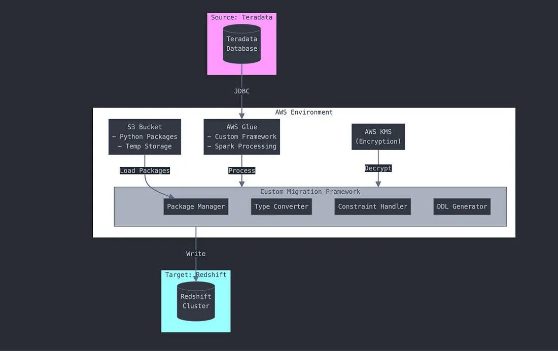
Core Migration Tools
Our solution leverages:
- AWS Glue for ETL processing
- Apache Spark for data transformation
- Custom Python packages loaded from S3
- JDBC connections for direct database access
Data Migration Steps
- Extract Schema Information:
The process begins by extracting schema information from the source Teradata database. This is done using the get_jdbc_data function, which retrieves the column definitions for the specified database and table:
ddl_info = get_jdbc_data(spark, source_jdbc_conf, db, tb, ddl_info='Columns')
- The get_jdbc_data function connects to Teradata using JDBC (Java Database Connectivity). When ddl_info=’Columns’, it queries Teradata’s system tables (DBC.ColumnsV).
- Returns metadata including: column names, data types, column lengths, precision and scale for numeric types, nullable flags, and default values.
2. Map Data Types:
The extracted schema information is then used to map Teradata data types to their corresponding Amazon Redshift data types. This is crucial to ensure compatibility between the source and target systems:
mapped_columns, unord_columns = map_teradata_to_redshift(ddl_info)
- The map_teradata_to_redshift processes each column from the ddl_info
- For each column, it: Looks up the equivalent Redshift data type. Handles special cases (like DECIMAL with precision/scale). Preserves NULL/NOT NULL constraints. Maintains column formatting
- Returns: mapped_columns List of fully formatted columns with Redshift types. unord_columns Dictionary mapping column names to their base Redshift types.
3. Create Target Tables:
Using the mapped schema, the target table is created in Redshift. The create_redshift_ddl function generates the Data Definition Language (DDL) statements required for table creation:
redshift_ddl = create_redshift_ddl('xyz', db[4:].lower(), tb, ordered_columns)
This phase builds and creates the target table:
create_redshift_ddl:
- Constructs a CREATE TABLE statement
- Uses db[4:].lower() to format database name (e.g., “ASD_WER” → “wer”)
- Includes all columns with their mapped types
- Adds constraints (primary keys, unique constraints)
- ordered_columns ensures the columns are properly structured for the target table.
redshift_ddl_execute:
- Connects to Redshift using AWS’s redshift-data API
- Executes the DDL statement
- Handles any execution errors
redshift_ddl_execute(redshift_ddl)
- Transfer Data:
After the target table is created, the actual data transfer occurs. The data from Teradata is written to Redshift using the write_data function:
write_data(dynamic_frame, glueContext, db[4:].lower(), tb)
Here, dynamic_frame represents the data in a schema-flexible format, which is written to the target Redshift table using AWS Glue’s glueContext. The db[4:].lower() parameter ensures the target database name adheres to the expected naming convention.
Uses AWS Glue’s DynamicFrame (more flexible than Spark DataFrame)
The write_data function: Sets up connection to Redshift
- Configures write options (like temporary S3 storage)
- Handles data type conversions automatically
- Manages the bulk data transfer process
- Uses Redshift’s COPY command under the hood for efficient loading
Edge Cases and Solutions
Here are some other edge cases that could potentially cause issues during your migration:
Unmapped Data Types: Unmapped types can disrupt migration. The warning mechanism helps detect and address these early.
Data Type Complexity: Complex types like INTERVAL or TIME WITH TIME ZONE require additional logic for accurate handling.Custom logic for various interval types (YEAR TO MONTH, DAY TO SECOND). Timezone Management which preserves timezone information while handling FORMAT differences and special handling for BYTE, VARBYTE, and BLOB data (Binary Types).
Default Value Handling: Improper default handling can cause inconsistencies. Rigorous testing ensures alignment with Redshift’s expectations. Proper management of NULL vs NOT NULL constraints.
Dynamic Length and Precision: Handling dynamic lengths and precision from incomplete metadata is tricky. Robust logic ensures accurate data representation. Analyzes data patterns to optimize column lengths and prevents data truncation.
1. Complex Data Types
Teradata uses several data types that don’t have direct equivalents in Redshift, particularly:
- PERIOD data types (PD, PS, PT, PZ)
- Interval types (DH, DM, DS, HM, HR)
- Binary types (BF, BO, BV)
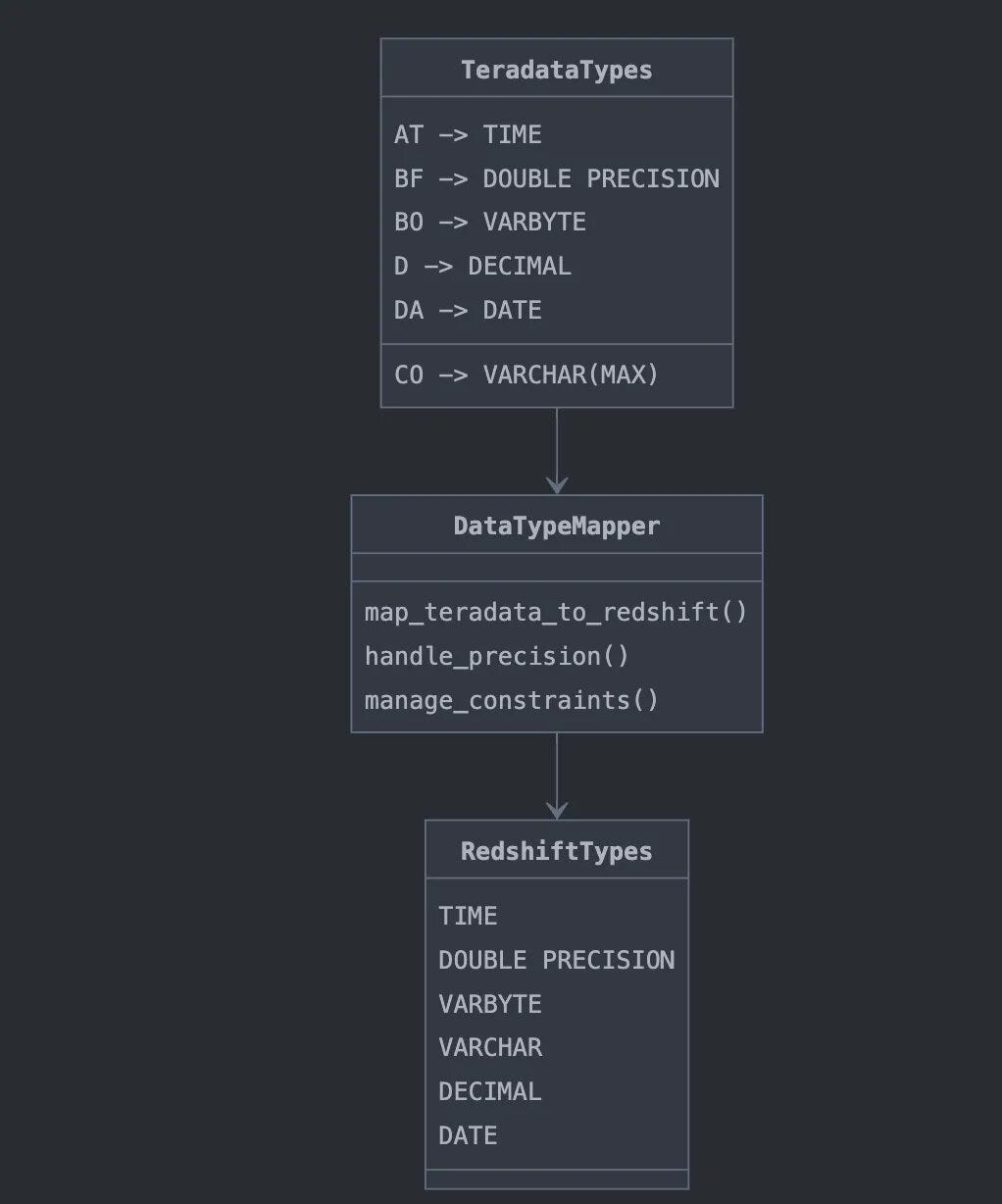
teradata_to_redshift_datatype = {
    "AT": "TIME",     # ANSI Time
    "BF": "DOUBLE PRECISION", # Byte Float
    "BO": "VARBYTE", # Byte Large Object
    "BV": "VARBYTE", # Byte Varying
    "CF": "CHAR",    # Character (Fixed)
    "CO": "VARCHAR(MAX)", # Character Large Object
    "CS": "VARCHAR", # Character Set
    "CV": "VARCHAR", # Character Varying
    "D": "DECIMAL",
    "DA": "DATE",
    "DH": "INTERVAL DAY TO HOUR",
    "DM": "INTERVAL DAY TO MINUTE",
    "DS": "INTERVAL DAY TO SECOND",
    "DY": "INTERVAL DAY",
    "F": "FLOAT",
    "HM": "INTERVAL HOUR TO MINUTE",
    "HR": "INTERVAL HOUR",
    "HS": "INTERVAL HOUR TO SECOND",
    "I": "INTEGER",
    "I1": "SMALLINT", # 1-byte integer
    "I2": "SMALLINT", # 2-byte integer
    "IB": "BIGINT",   # 8-byte integer
    "MI": "INTERVAL MINUTE",
    "MO": "INTERVAL MONTH",
    "MS": "INTERVAL MINUTE TO SECOND",
    "N": "DECIMAL",   # Exact numeric
    "PD": "TIMESTAMP", # Period (DATE)
    "PM": "INTERVAL YEAR TO MONTH",
    "PS": "TIMESTAMP", # Period (TIMESTAMP)
    "PT": "TIME",     # Period(TIME)
    "PZ": "TIMESTAMPTZ", # Period (TIMESTAMP WITH TIME ZONE)
    "SC": "INTERVAL SECOND",
    "SZ": "TIMESTAMPTZ", # Timestamp with time zone
    "TS": "TIMESTAMP", # Timestamp
    "TZ": "TIMETZ",   # Time with time zone
    "YI": "INTERVAL YEAR",
    "YM": "INTERVAL YEAR TO MONTH",
    "UT": "VARCHAR"   # User-defined type
}
2. Constraint Preservation
Redshift doesn’t support foreign key constraints, and primary key constraints are handled differently than in Teradata.
We implemented custom constraint handling:
def get_constraints(df):
    constr_map, primary_indexes, second_indexes = {}, {}, []
    for row in df.collect():
        column_name, index_name = row.ColumnName, row.IndexName
        if index_name in constr_map:
            constr_map[index_name].append(column_name)
        else:
            constr_map[index_name] = [column_name]

    for index_name, column_list in constr_map.items():
        if len(column_list) == 1:
            primary_indexes[column_list[0]] = index_name
        else:
            strr = f'constraint {index_name} unique ('
            for column in column_list:
                strr += column + ','
            strr = strr[:-1] + ')'
            second_indexes.append(strr)

    return constr_map, primary_indexes, second_indexes
3. Large Dataset Handling
Migrating large tables can notoriously lead to memory issues and timeout problems. To handle that we implemented batch processing using Spark and AWS Glue:
def write_data(dynamic_frame, glue_context, schema, table_name):
    connection = glue_context.extract_jdbc_conf(
        'glue-to-redshift-connectionname'
    )
    database_name = connection['fullUrl'].split('/')[-1]
    my_conn_options = {
        "dbtable": f"{schema}.{table_name}",
        "database": database_name,
        "useConnectionProperties": "true",
        "connectionName": "glue-to-redshift-connectionname"
    }

    temp_dir = "s3://qwe-temp/abc/"

    glue_context.write_dynamic_frame.from_jdbc_conf(
        frame=dynamic_frame,
        catalog_connection="glue-to-redshift-connectionname",
        connection_options=my_conn_options,
        redshift_tmp_dir=temp_dir
    )
Conclusion
Our journey building a custom migration framework demonstrates that enterprise-scale migrations often require solutions beyond standard tools. By leveraging AWS Glue, PySpark, and custom Python implementations, we’ve created a framework that effectively handles complex data types, preserves constraints, and provides the precise control that large-scale migrations demand.
The framework serves as a blueprint for teams facing similar challenges, proving that even complex database migrations can be automated and streamlined. While AWS’s native tools provide a solid foundation, our approach offers the flexibility and robustness required for enterprise deployments. As organizations continue modernizing their data infrastructure, frameworks like this become essential for executing controlled, efficient, and reliable database migrations at scale.